CplexA tutorial (Mathematica implementation)
Jose M. G. Vilar and Leonor Saiz
 Biophysics Unit (CSIC-UPV/EHU) and Department of Biochemistry and Molecular Biology, University of the Basque Country, P.O. Box 644, 48080 Bilbao, Spain
 IKERBASQUE, Basque Foundation for Science, 48011 Bilbao, Spain
 Department of Biomedical Engineering, University of California, 451 East Health Sciences Drive, Davis, CA 95616, USA
SUMMARY: CplexA is a software package (available for Mathematica, Python, and Matlab) to study the effects of macromolecular assembly on cellular processes. A main challenge for conventional computational methods to study macromolecular assembly is tackling the exponential increase of the number of configurational states with the number of components. CplexA uses functional programming to efficiently compute probabilities and average properties over such exponentially large number of states from the energetics of the interactions. The package is particularly suited to study gene expression at complex promoters controlled by multiple, local and distal, DNA binding sites for transcription factors. CplexA is freely available at http://sourceforge.net/projects/cplexa/.
REFERENCES:
1) The main reference for CplexA is Vilar, J.M.G. and Saiz, L. (2010) CplexA: a Mathematica package to study macromolecular-assembly control of gene expression, Bioinformatics 26, 2060-2061.
2) The biophysical background of the methods used by CplexA are described in Saiz, L. and Vilar, J.M.G. (2006) Stochastic dynamics of macromolecular-assembly networks, Mol Syst Biol, 2, 2006.0024.
Running the tutorial
To run the tutorial the file CplexA.m must be in the Path, the default list of directories searched by Mathematica to find an external file. A possibility is to place CplexA.m in the same directory as the tutorial notebook.


The main function of CplexA is AvConf[Γ, ΔG, S, RT]= (∑Γ )/(∑
)/(∑ ), which efficiently computes the thermodynamic average of Γ for a system with free energy ΔG described by the set S of state variables. Each state variable can take the values 0 or 1 to represent whether a property is present or not. Both Γ and ΔG are functions of S. RT is the thermal energy (gas constant, R, times the absolute temperature, T). The sums are performed over all possible combinations of values of the state variables.
Note that different units can be used for the thermal energy, for instance kT (AvConf[Γ, ΔG, S, kT]) or even numerical values explicitly (AvConf[Γ, ΔG, S, 0.6]). The three-argument function AvConf[Γ, ΔG, S] assumes the default thermal energy, which is set initially to RT. The default thermal energy can be changed with the function SetTE[default_value], as for instance SetTE[kT], SetTE[0.6], or SetTE[RT].
CplexA also implements the function AvConfF[Γ, ΔG, S, RT], which produces the same results as AvConf[Γ, ΔG, S, RT], but uses a slightly different algorithm to compute the sums. It is slower than AvConf for small systems but sometimes can be faster for large systems.
Using CplexA it is also possible to follow the traditional approach where a table provides the free energies and probabilities of all the possible configurations of the complex. The function DGTable[ΔG, S, RT] of CplexA constructs a table with the free energy and statistical weight (Boltzmann factor) of each state that has a non-zero probability.
An activator
A transcription factor with concentration n1 binds a DNA site described by the state variable s1. The variable indicates whether (s1=1) or not (s1=0) the transcription factor is bound. S is the set of state variables describing the system (in this case, it consists only of s1); ΔG is the free energy of the system; ΔG° is the standard free energy of binding at 1M; and Γ is the transcription rate, which is Γmax when the transcription factor is bound (s1=1) or zero when it is not (s1=0).
The example below computes the average transcription rate AΓ.


Same example as before, but now the free energy is expressed in terms of the dissociation constant Kd (recall the equivalency Kd= ):
):


Two molecules binding to overlapping sites
Two molecules with concentrations n1 and n2 compete for binding to overlapping sites (binding of one excludes the binding of the other). The variables s1 and s2 indicate whether molecules 1 and 2 are bound, respectively. The expression below computes the probability that molecule 1 is bound, which is given by the average value of s1.
Note the term ∞ s1 s2 in the free energy. It implements the logical condition that two molecules cannot be bound simultaneously by assigning an infinite free energy to the corresponding state. To obtain the correct thermodynamic result, the symbol ∞ is considered to be finite until the end result, and then the limit to infinity is taken.


CplexA also provides the function DGTable[ΔG, S, RT], which constructs a table with the free energy and statistical weight (Boltzmann factor) of each state that has a non-zero probability. For the previous example, it is used as follows:

Cooperative binding
Similar to the previous example, but now the binding of one does not exclude the other. The term e12 is the interaction energy between the molecules bound. The following expression computes the probability of having the two sites occupied simultaneously:


The function DGTable[ΔG, S, RT] can be used here to construct the free energy and statistical weight table for cooperative binding:

lac Operon
The lac repressor is a protein with two DNA binding domains. It can bind to one site or, by looping the intervening DNA, to two distal sites simultaneously.
In addition to the domain-binding state variables to each site, s1 and s2, there is a looping state variable sL that indicates wether the DNA is looped (sL=1) or not (sL=0). Note that the each binding domain at sites 1 and 2 can be from two different lac repressors or from a single one when there is looping. The term ∞ (1 - s1 s2) sL means that looping can only happen with two domains bound, otherwise the free energy is infinite.
The following expression computes the repression level:


Note that gL is the contribution to the free energy due to the conformational change of DNA (free energy of looping).
The following expression constructs the table for the free energies and statistical weights for the binding of the lac repressor to two DNA binding sites:

Phage λ
The CI protein of phage λ can bind as a dimer to three sites on the right operator (described here by the state variables sOR1, sOR2, and sOR3 ) and to another three sites on the left operator (described by sOL1, sOL2, and sOL3). The state variable sL describes the looping state.
The free energy of the system ΔGλ takes into account interactions between CI dimers bound at neighboring sites and, when there is looping (sL=1), at different operators as well.


Transcription at the PRM promoter is given by Γrm, which leads to the average AΓrm. There is also another promoter, PR, with transcription given by Γr, which leads to the average AΓr.


Note that in both cases it is possible to obtain an exact analytical expression for the effective transcription rates, AΓrm and AΓr, as a function of the CI dimer concentration. The expression NF below gives the CI dimer concentration as function of the normalized CI monomer concentration.

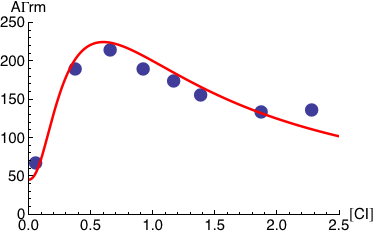
Plotted below is AΓrm (solid red line) as a function of the normalized CI monomer concentration. The filled circles correspond the experimentally measured activity of the PRM promoter (Dodd, I.B., Shearwin, K.E., Perkins, A.J., Burr, T., Hochschild, A.and Egan, J.B.(2004) Cooperativity in longrange gene regulation by the lambda CI repressor, Genes Dev, 18, 344-354).


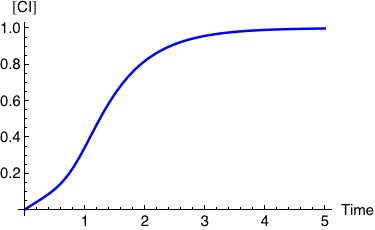
The expression below computes and plots the kinetics of the normalized CI concentration starting from [CI]=0 until it reaches its saturation value. It assumes that the production of CI is proportional to the transcriptional activity, AΓrm, and that the degradation rate of CI is equal to 1.


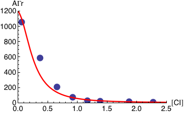
Plotted below is AΓr (solid red line) as a function of the normalized CI monomer concentration. The filled circles correspond the experimentally measured activity of the PR promoter ( Dodd, I.B., Shearwin, K.E., Perkins, A.J., Burr, T., Hochschild, A.and Egan, J.B.(2004) Cooperativity in longrange gene regulation by the lambda CI repressor, Genes Dev, 18, 344 - 354).


In this case, CplexA is able to provide with a few lines of code results that would require writing tables with 128 entries, one for each binding state, with traditional thermodynamic approaches, as shown below.

|
ΔG |
 |
 |
|
0 |
1 |
 |
|
21 |
 |
 |
|
-10.2-RT Log[n] |
 |
 |
|
10.8-RT Log[n] |
 |
 |
|
-10.7-RT Log[n] |
 |
 |
|
10.3-RT Log[n] |
 |
 |
|
-23.9-2 RT Log[n] |
 |
 |
|
-2.9-2 RT Log[n] |
 |
 |
|
-12.7-RT Log[n] |
 |
 |
|
8.3-RT Log[n] |
 |
 |
|
-22.9-2 RT Log[n] |
 |
 |
|
-1.9-2 RT Log[n] |
 |
 |
|
-26.4-2 RT Log[n] |
 |
 |
|
-5.4-2 RT Log[n] |
 |
 |
|
-36.6-3 RT Log[n] |
 |
 |
|
-15.6-3 RT Log[n] |
 |
 |
|
-12.4-RT Log[n] |
 |
 |
|
8.6-RT Log[n] |
 |
 |
|
-22.6-2 RT Log[n] |
 |
 |
|
-4.6-2 RT Log[n] |
 |
 |
|
-23.1-2 RT Log[n] |
 |
 |
|
-2.1-2 RT Log[n] |
 |
 |
|
-36.3-3 RT Log[n] |
 |
 |
|
-18.3-3 RT Log[n] |
 |
 |
|
-25.1-2 RT Log[n] |
 |
 |
|
-4.1-2 RT Log[n] |
 |
 |
|
-35.3-3 RT Log[n] |
 |
 |
|
-17.3-3 RT Log[n] |
 |
 |
|
-38.8-3 RT Log[n] |
 |
 |
|
-17.8-3 RT Log[n] |
 |
 |
|
-49.-4 RT Log[n] |
 |
 |
|
-31.-4 RT Log[n] |
 |
 |
|
-12.1-RT Log[n] |
 |
 |
|
8.9-RT Log[n] |
 |
 |
|
-22.3-2 RT Log[n] |
 |
 |
|
-1.3-2 RT Log[n] |
 |
 |
|
-22.8-2 RT Log[n] |
 |
 |
|
-1.8-2 RT Log[n] |
 |
 |
|
-36.-3 RT Log[n] |
 |
 |
|
-15.-3 RT Log[n] |
 |
 |
|
-24.8-2 RT Log[n] |
 |
 |
|
-3.8-2 RT Log[n] |
 |
 |
|
-35.-3 RT Log[n] |
 |
 |
|
-14.-3 RT Log[n] |
 |
 |
|
-38.5-3 RT Log[n] |
 |
 |
|
-17.5-3 RT Log[n] |
 |
 |
|
-48.7-4 RT Log[n] |
 |
 |
|
-27.7-4 RT Log[n] |
 |
 |
|
-27.-2 RT Log[n] |
 |
 |
|
-6.-2 RT Log[n] |
 |
 |
|
-37.2-3 RT Log[n] |
 |
 |
|
-19.2-3 RT Log[n] |
 |
 |
|
-37.7-3 RT Log[n] |
 |
 |
|
-16.7-3 RT Log[n] |
 |
 |
|
-50.9-4 RT Log[n] |
 |
 |
|
-32.9-4 RT Log[n] |
 |
 |
|
-39.7-3 RT Log[n] |
 |
 |
|
-18.7-3 RT Log[n] |
 |
 |
|
-49.9-4 RT Log[n] |
 |
 |
|
-31.9-4 RT Log[n] |
 |
 |
|
-53.4-4 RT Log[n] |
 |
 |
|
-32.4-4 RT Log[n] |
 |
 |
|
-63.6-5 RT Log[n] |
 |
 |
|
-45.6-5 RT Log[n] |
 |
 |
|
-13.8-RT Log[n] |
 |
 |
|
7.2-RT Log[n] |
 |
 |
|
-24.-2 RT Log[n] |
 |
 |
|
-3.-2 RT Log[n] |
 |
 |
|
-24.5-2 RT Log[n] |
 |
 |
|
-3.5-2 RT Log[n] |
 |
 |
|
-37.7-3 RT Log[n] |
 |
 |
|
-16.7-3 RT Log[n] |
 |
 |
|
-26.5-2 RT Log[n] |
 |
 |
|
-5.5-2 RT Log[n] |
 |
 |
|
-36.7-3 RT Log[n] |
 |
 |
|
-15.7-3 RT Log[n] |
 |
 |
|
-40.2-3 RT Log[n] |
 |
 |
|
-19.2-3 RT Log[n] |
 |
 |
|
-50.4-4 RT Log[n] |
 |
 |
|
-29.4-4 RT Log[n] |
 |
 |
|
-26.2-2 RT Log[n] |
 |
 |
|
-5.2-2 RT Log[n] |
 |
 |
|
-36.4-3 RT Log[n] |
 |
 |
|
-18.4-3 RT Log[n] |
 |
 |
|
-36.9-3 RT Log[n] |
 |
 |
|
-15.9-3 RT Log[n] |
 |
 |
|
-50.1-4 RT Log[n] |
 |
 |
|
-32.1-4 RT Log[n] |
 |
 |
|
-38.9-3 RT Log[n] |
 |
 |
|
-17.9-3 RT Log[n] |
 |
 |
|
-49.1-4 RT Log[n] |
 |
 |
|
-31.1-4 RT Log[n] |
 |
 |
|
-52.6-4 RT Log[n] |
 |
 |
|
-31.6-4 RT Log[n] |
 |
 |
|
-62.8-5 RT Log[n] |
 |
 |
|
-44.8-5 RT Log[n] |
 |
 |
|
-28.4-2 RT Log[n] |
 |
 |
|
-7.4-2 RT Log[n] |
 |
 |
|
-38.6-3 RT Log[n] |
 |
 |
|
-17.6-3 RT Log[n] |
 |
 |
|
-39.1-3 RT Log[n] |
 |
 |
|
-18.1-3 RT Log[n] |
 |
 |
|
-52.3-4 RT Log[n] |
 |
 |
|
-31.3-4 RT Log[n] |
 |
 |
|
-41.1-3 RT Log[n] |
 |
 |
|
-20.1-3 RT Log[n] |
 |
 |
|
-51.3-4 RT Log[n] |
 |
 |
|
-30.3-4 RT Log[n] |
 |
 |
|
-54.8-4 RT Log[n] |
 |
 |
|
-55.-4 RT Log[n] |
 |
 |
|
-65.-5 RT Log[n] |
 |
 |
|
-65.2-5 RT Log[n] |
 |
 |
|
-40.8-3 RT Log[n] |
 |
 |
|
-19.8-3 RT Log[n] |
 |
 |
|
-51.-4 RT Log[n] |
 |
 |
|
-33.-4 RT Log[n] |
 |
 |
|
-51.5-4 RT Log[n] |
 |
 |
|
-30.5-4 RT Log[n] |
 |
 |
|
-64.7-5 RT Log[n] |
 |
 |
|
-46.7-5 RT Log[n] |
 |
 |
|
-53.5-4 RT Log[n] |
 |
 |
|
-32.5-4 RT Log[n] |
 |
 |
|
-63.7-5 RT Log[n] |
 |
 |
|
-45.7-5 RT Log[n] |
 |
 |
|
-67.2-5 RT Log[n] |
 |
 |
|
-67.4-5 RT Log[n] |
 |
 |
|
-77.4-6 RT Log[n] |
 |
 |
|
-80.6-6 RT Log[n] |
 |
 |


